Exact and heuristic methods for tearing
Many of the implemented algorithms are described in the following academic papers (submitted, only drafts are available on these links):
See also Reproducing the results of the academic papers.
The source code of the prototype implementation is
available on GitHub
under the 3-clause BSD license. The code is a work in progress. Some of the code
will be contributed back to
NetworkX
wherever it is appropriate. The remaining part of the code will be released as a
Python package on PyPI. In the meantime, the rpc_api.py is a good place
to start looking. (rpc stands for remote procedure call; it can be
called from Java or C++ through the json_io.py) The API in
rpc_api.py takes a sparse matrix in coordinate format and returns the
row and column permutation vectors. As for the rest of this web-page, a demo
application demo.py is presented here, showing the capabilities of the
novel tearing algorithms.
Sparse matrices ordered to spiked form
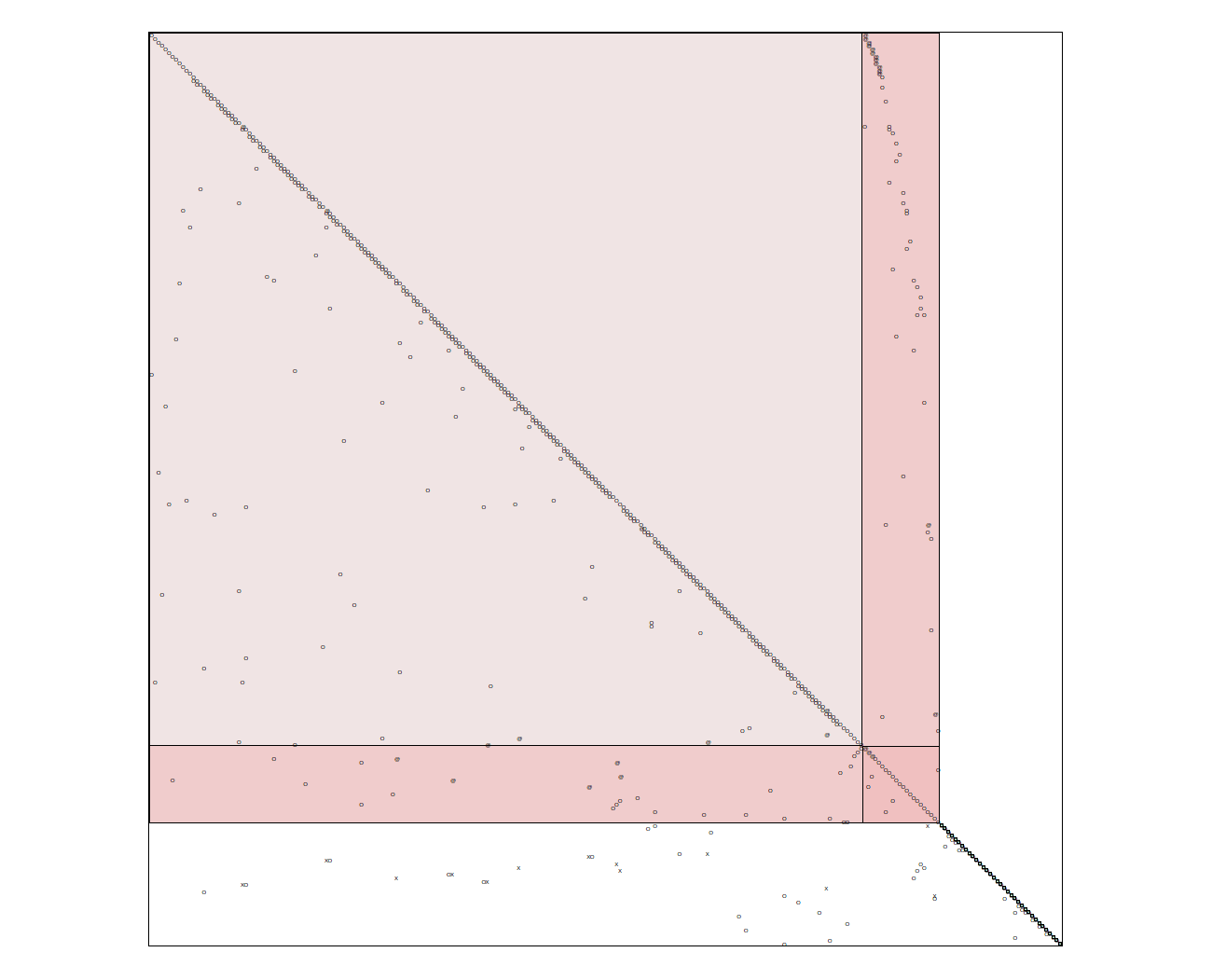
Roughly speaking, tearing algorithms rearrange the rows and the columns of a sparse matrix in such a way that the result is “close” to a lower triangular matrix. A sparse matrix ordered to the so-called spiked form is shown in the picture below. The matrix is of size 76x76; it can be reduced to a 5x5 matrix by elimination, where 5 equals the number of spike columns, that is, columns with red entries. The blue lines correspond to the device boundaries in the technical system; the tear variables are above the diagonal, and are painted red; the gray squares are “forbidden” variables (no explicit elimination possible). The elimination is performed along the diagonal.
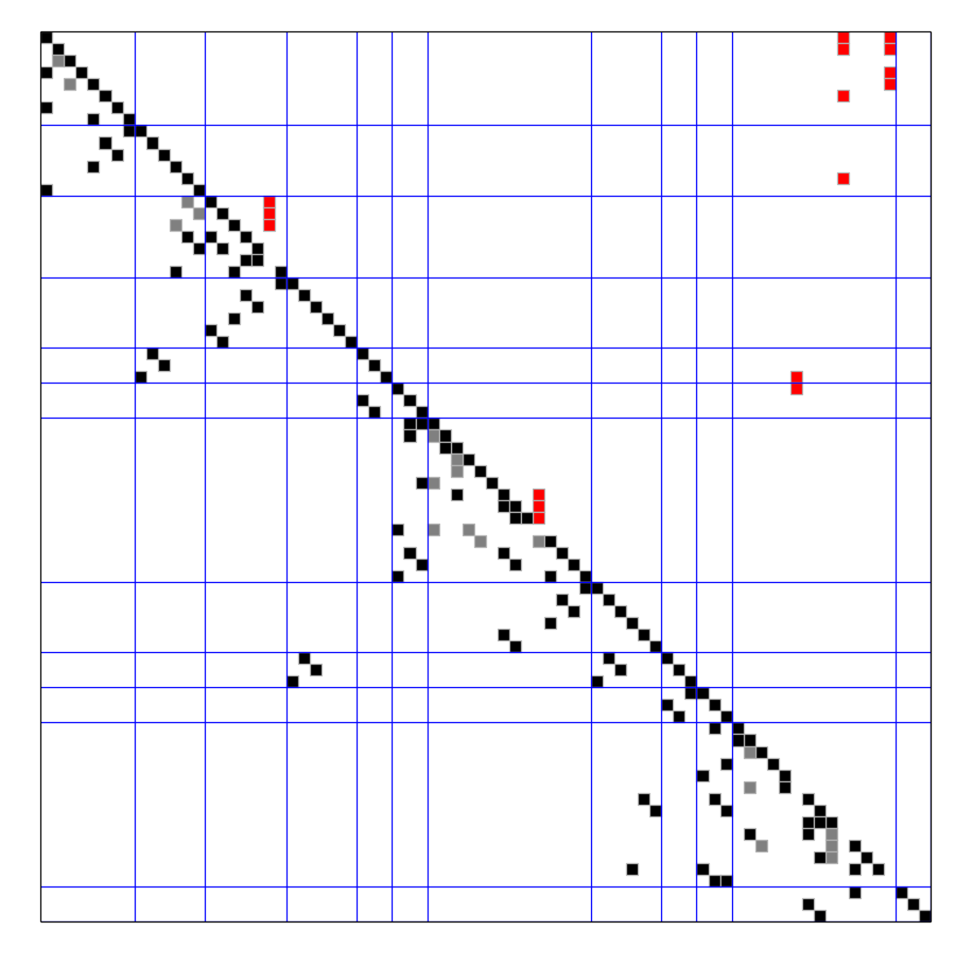
A sparse matrix ordered to the so-called spiked form
Steps of the demo application
You find the source code of the demo application in demo.py.
1. Input: flattened Modelica model
The Modelica model data/demo.mo has
already been flattened with the JModelica
compiler by calling compile_fmux(); check the flatten and
fmux_creator modules for details. The demo application takes the
flattened model as input. The OpenModelica Compiler can also emit the necessary
XML file, see under Export > Export XML in OMEdit; unfortunately, it is
unclear how to disable alias variable elimination and tearing in this compiler.
2. Recovering the process graph
A directed graph is recovered from the flattened model: The devices correspond to the vertices of the process graph, the edges correspond to the material flows.
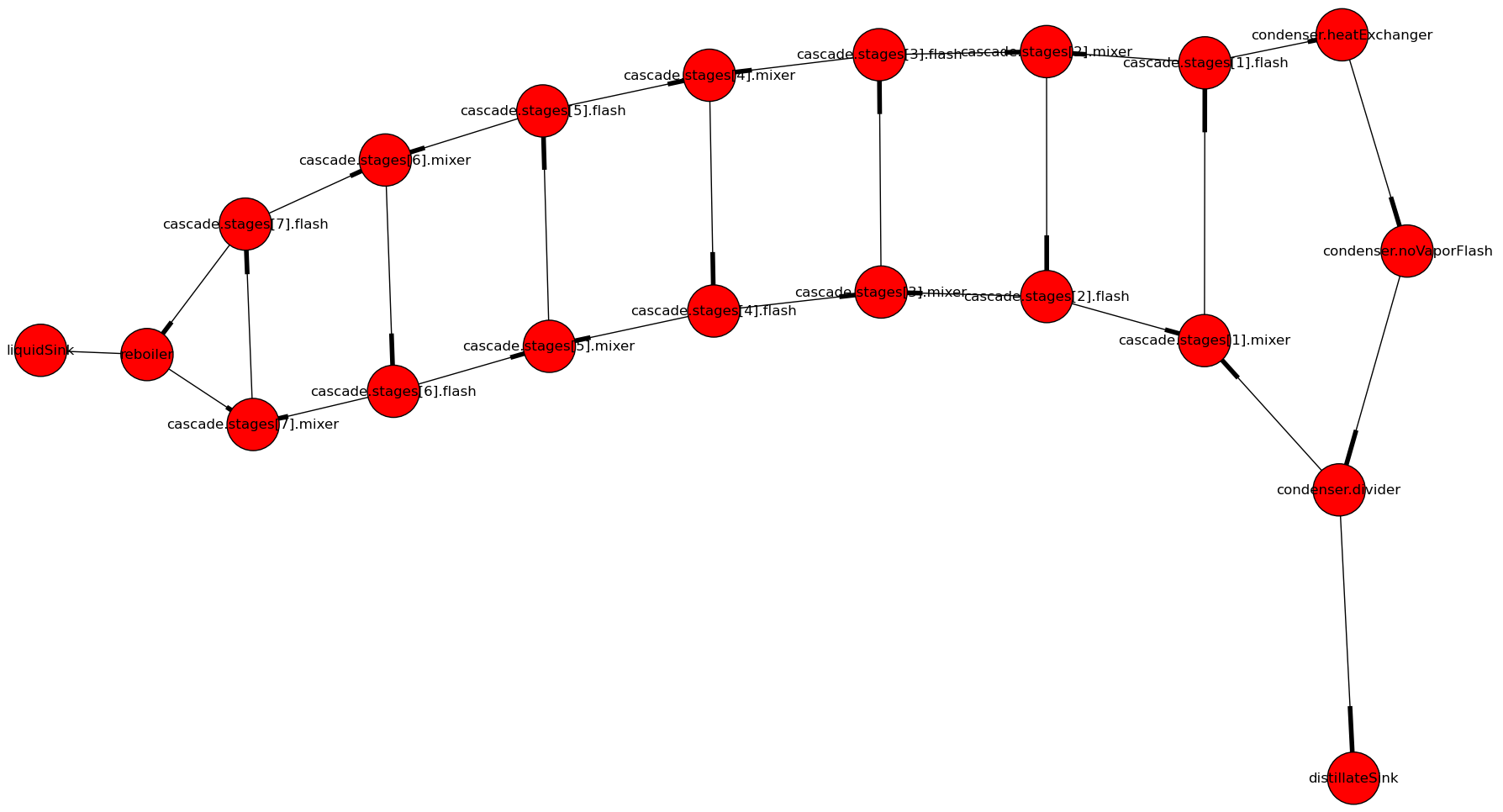
The process graph of a distillation column with 7 stages (click on the image to enlarge it)
The process graph is used for partitioning the Jacobian of the system of equations: This is how the blue lines in the first picture were obtained.
At the moment, recovering the directed edges is possible only if the input
connectors of the devices are called inlet, and their output connectors
are called outlet. There is an ongoing discussion with the JModelica
developers on reconstructing the process graph in a generic way, without
assuming any naming convention for the connectors.
3. Symbolic manipulation of the equations
The equations are given as binary expression trees in the input flattened Modelica model.

The expression tree of y = alpha*x/(1+(alpha-1)*x) in SymPy
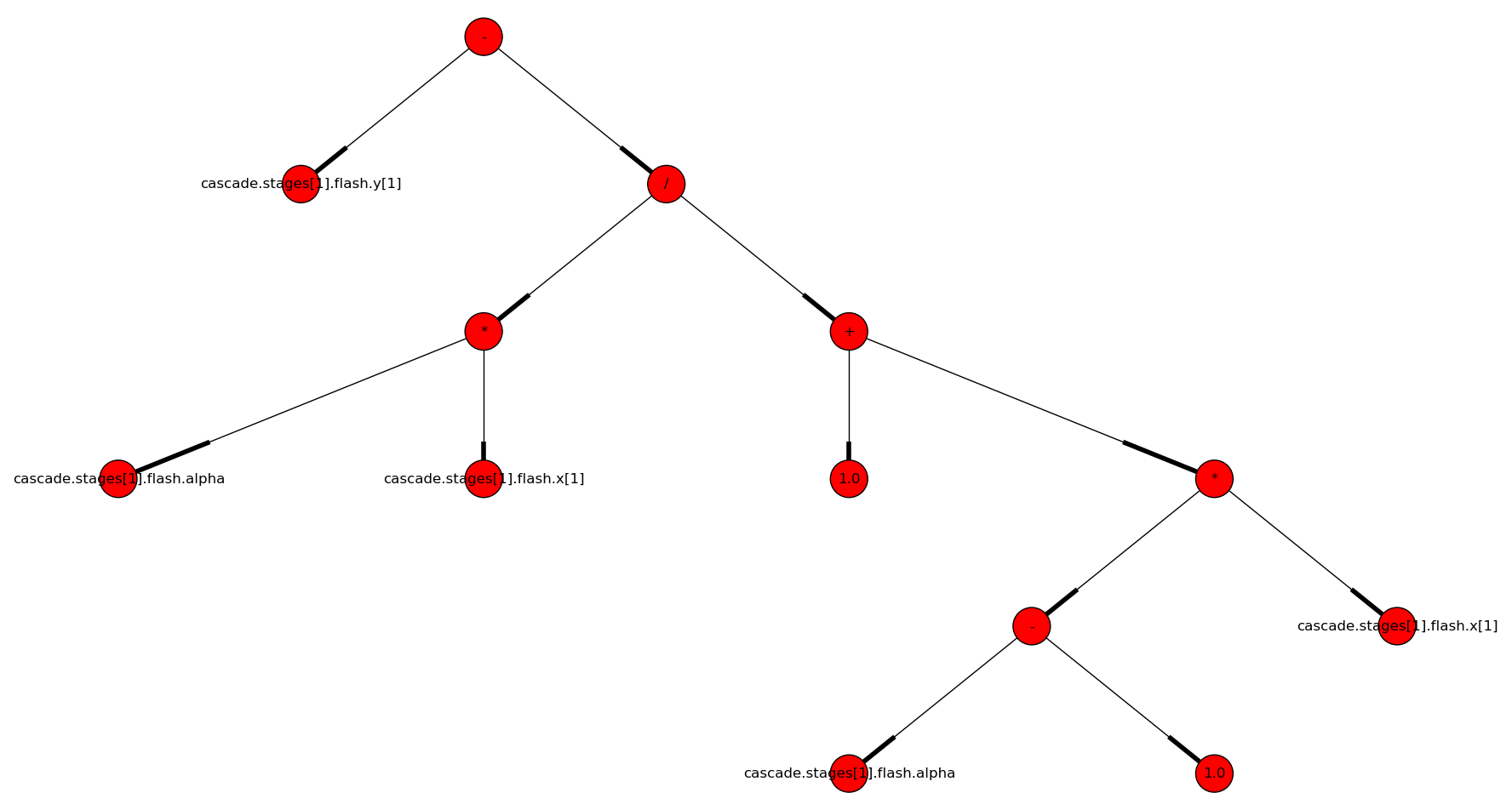
The same expression tree of y = alpha*x/(1+(alpha-1)*x))
but as a NetworkX DiGraph
The expression trees of the equations are symbolically manipulated with SymPy to determine which variables can be explicitly and
safely eliminated from which equations. An example for unsafe elimination is
the rearrangement of x*y=1 to y=1/x if x may potentially take on the
value 0. Unsafe eliminations are automatically recognized and avoided; these
were the gray entries in the first picture.
4. Optimal tearing
There is no clear objective for tearing. A common choice is to minimize the size of the final reduced system, or in other words, to minimize the number of spike columns. Although this objective is questionable (it ignores numerical stability for example), it nevertheless makes the meaning of optimal mathematically well-defined.
If Gurobi is installed, the Jacobian is ordered optimally with an exact method, based on integer programming. For the same system that was shown in the first picture, we get an optimal ordering that yields a 4x4 reduced system. The suboptimal ordering shown in the first picture gives a 5x5 reduced system, and was obtained with the heuristic method detailed in the next section. The integer programming approach does not need or use the block structure which was given with the blue lines in the first picture; here the blue lines are absent.
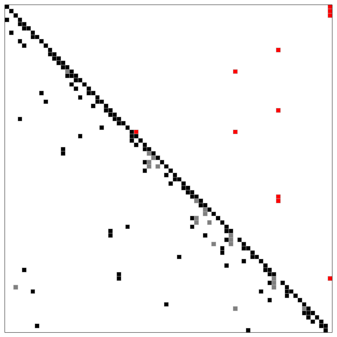
Optimal order, obtained with integer programming
Note that the first spike is the red entry right above the diagonal.
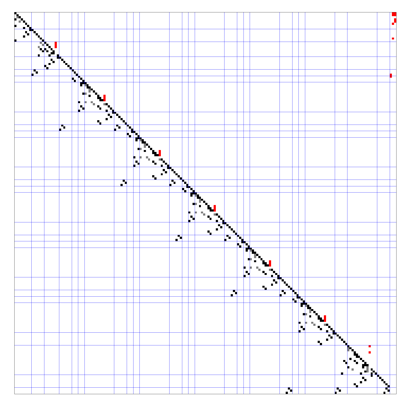
5. A hierarchical tearing heuristic exploiting the natural block structure
Technical systems can be partitioned into blocks along the device boundaries in a fairly natural way. We call this partitioning the natural block structure. The implemented tearing heuristic first orders the blocks, then the equations within each block. This is how the first picture with the spiked form was obtained. Exactly the same picture is shown below for your convenience.
Hierarchical tearing with the natural block structure
Further details are discussed in Tearing systems of nonlinear equations I. A survey under 7.3. Hierarchical tearing.
5.1 Tearing as seen in Modelica tools
First, the undirected bipartite graph representation of the system of equations is oriented with matching; in other words, the undirected graph is made directed. Then, the strongly connected components (SCC) of this directed graph are identified. This way of identifying the SCCs is also referred to as block lower triangular decomposition (BLT decomposition) or Dulmage-Mendelsohn decomposition. After finishing the BLT decomposition, a subset of the edges is torn within each SCC to make them acyclic. Greedy heuristics, for example variants of Cellier’s heuristic, are used to find a tear set with small cardinality. This approach can produce unsatisfactory results if the system has large strongly connected components. An example is shown below.
Tearing obtained from JModelica with generate_html_diagnostics (click to enlarge)
As it can be seen in this picture, the BLT decomposition gave one large block. This is not surprising, as the example is a distillation column. The border width of the largest block (the number of torn variables) is proportional to the size of the column. For a realistic column, this can become problematic.
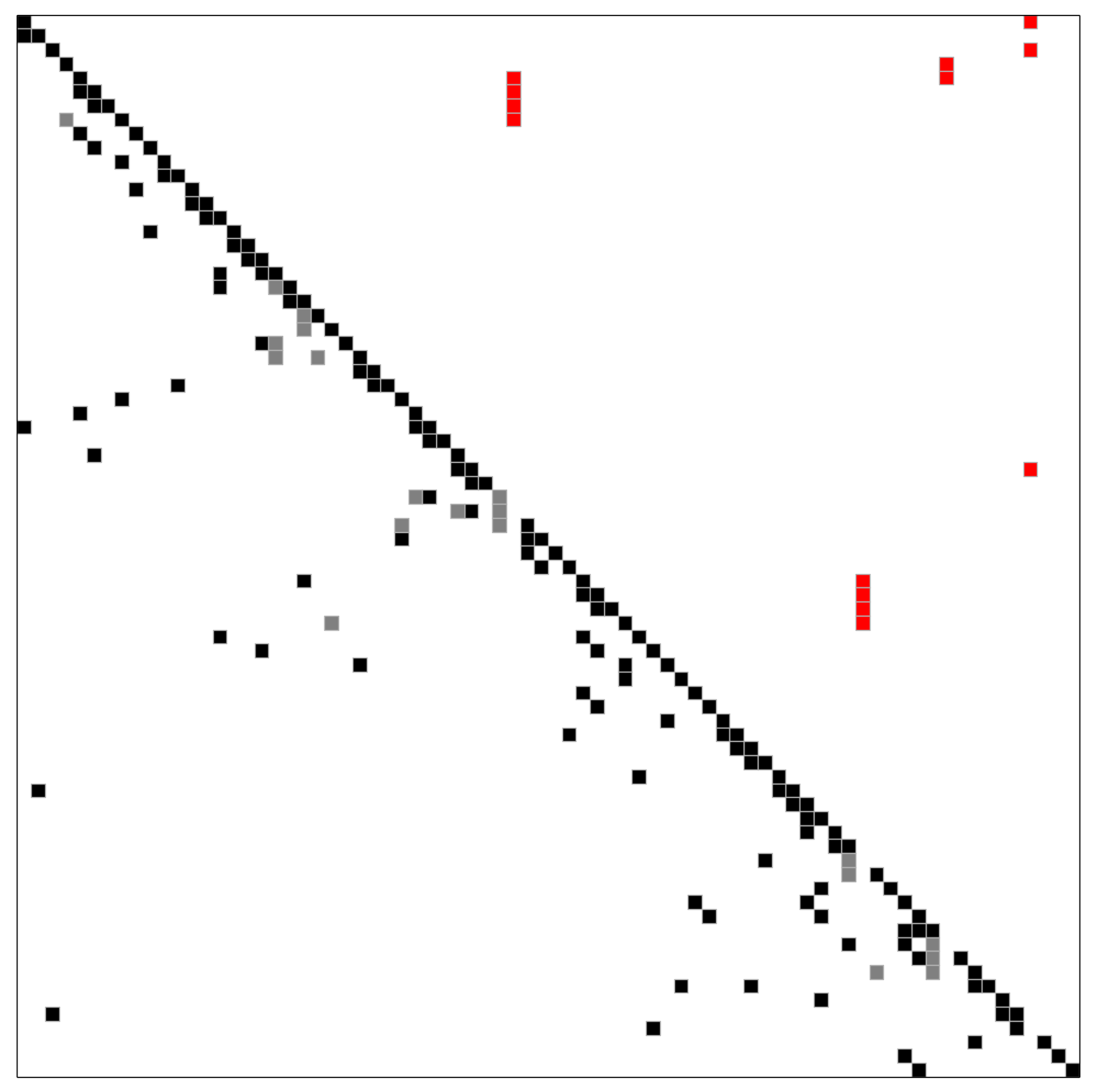
However, if the natural block structure is used for partitioning as discussed above, the number of torn variables (the border width) does not change with the size of the column. We get the following picture for exactly the same input.
Hierarchical tearing with the natural block structure (click to enlarge)
The first spike belongs to the condenser, then the next 5 spikes correspond to the 5 stages of the distillation column, and the reboiler comes last. The number of variables on the right border (3 spikes in this example) remains independent of the size of the column.
6. AMPL and Python code generation after tearing
Our ultimate goal is to reduce a large, sparse system of equations to a small one. To this end, AMPL code is generated in such a way that the variables can be eliminated as desired. After the elimination, the reduced system has as many variables and equations as the number of spike columns. An AMPL code snippet is shown below, generated with the demo application.
# Block
# Tears: condenser.divider.zeta (v19)
eq_14: v14 = v12*v19;  # condenser.divider.outlet[1].f[1] = condenser.divider.inlet[1].f[1]*condenser.divider.zeta
eq_15: v15 = v13*v19;  # condenser.divider.outlet[1].f[2] = condenser.divider.inlet[1].f[2]*condenser.divider.zeta
eq_16: v16 = v11*v19;  # condenser.divider.outlet[1].H = condenser.divider.inlet[1].H*condenser.divider.zeta
eq_17: v17 = v12 - v14;  # condenser.divider.outlet[2].f[1] = condenser.divider.inlet[1].f[1] - condenser.divider.outlet[1].f[1]
eq_18: v18 = v13 - v15;  # condenser.divider.outlet[2].f[2] = condenser.divider.inlet[1].f[2] - condenser.divider.outlet[1].f[2]
eq_19: ((v17*32.04)+(v18*60.1))-96.0 = 0;  # ((condenser.divider.outlet[2].f[1]*32.04)+(condenser.divider.outlet[2].f[2]*60.1))-96.0 = 0
eq_20: v20 = v11 - v16;  # condenser.divider.outlet[2].H = condenser.divider.inlet[1].H - condenser.divider.outlet[1].H
# Connections
eq_21: v21 = v20;  # cascade.stages[1].mixer.inlet[1].H = condenser.divider.outlet[2].H
eq_22: v22 = v17;  # cascade.stages[1].mixer.inlet[1].f[1] = condenser.divider.outlet[2].f[1]
eq_23: v23 = v18;  # cascade.stages[1].mixer.inlet[1].f[2] = condenser.divider.outlet[2].f[2]
eq_24: v24 = v16;  # distillateSink.inlet.H = condenser.divider.outlet[1].H
eq_25: v25 = v14;  # distillateSink.inlet.f[1] = condenser.divider.outlet[1].f[1]
eq_26: v26 = v15;  # distillateSink.inlet.f[2] = condenser.divider.outlet[1].f[2]
In the above code snippet, equations eq_14–eq_20 and variables
v14–v20 correspond to the third block on the diagonal, starting counting at the top left corner. Variable
v19 corresponds to the spike column of this third block. Equations
eq_21–eq_26 and variables v21–v26 correspond to the fourth
diagonal block with only black entries on its diagonal.
Executable Python code is also generated for evaluating the reduced system. The Python code only serves to cross-check correctness.
7. A greedy tearing heuristic
A greedy tearing heuristic has been implemented, inspired by algorithm (2.3) of Fletcher and Hall. The heuristic resembles the minimum degree algorithm, but it also works for highly unsymmetric matrices. The implemented heuristic does not need or use any block structure. When breaking ties in the greedy choice, a lookahead step can improve the quality of the ordering.
Spiked form obtained with the greedy tearing heuristic, no lookahead
There are five spikes without lookahead: The gray entry on the diagonal also counts as a spike.
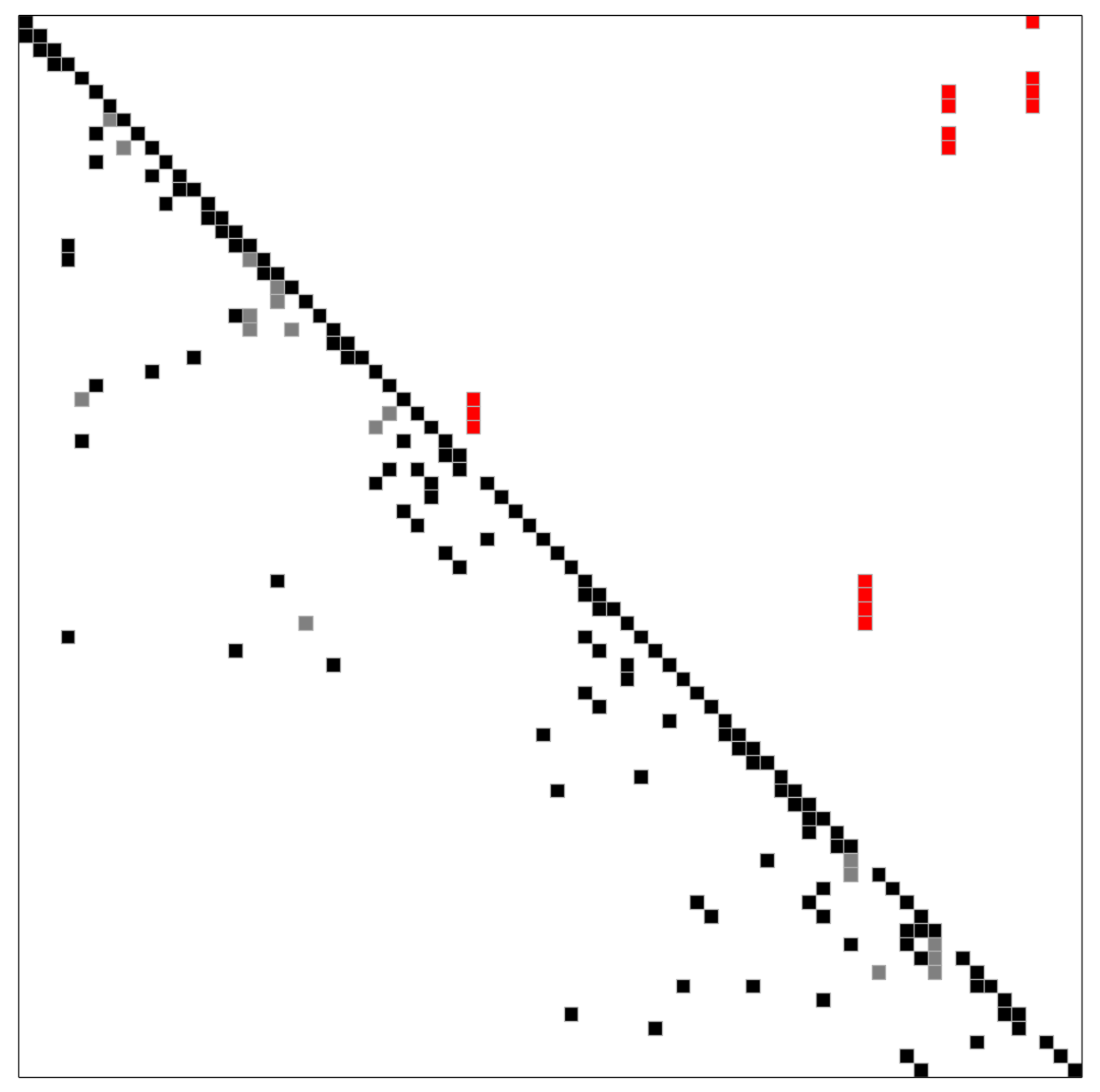
Spiked form obtained with the greedy tearing heuristic, happens to be optimal with lookahead
8. Tearing in chemical engineering
In abstract terms, this kind of tearing is equivalent to the minimum feedback arc set (MFAS) problem, the complement problem is known as the maximum acyclic subgraph problem. Compared to the tearing methods of Modelica tools, the differences are: (1) the graph is already oriented (directed), and (2) the nodes of the graph correspond to small systems of equations in the MFAS problem.
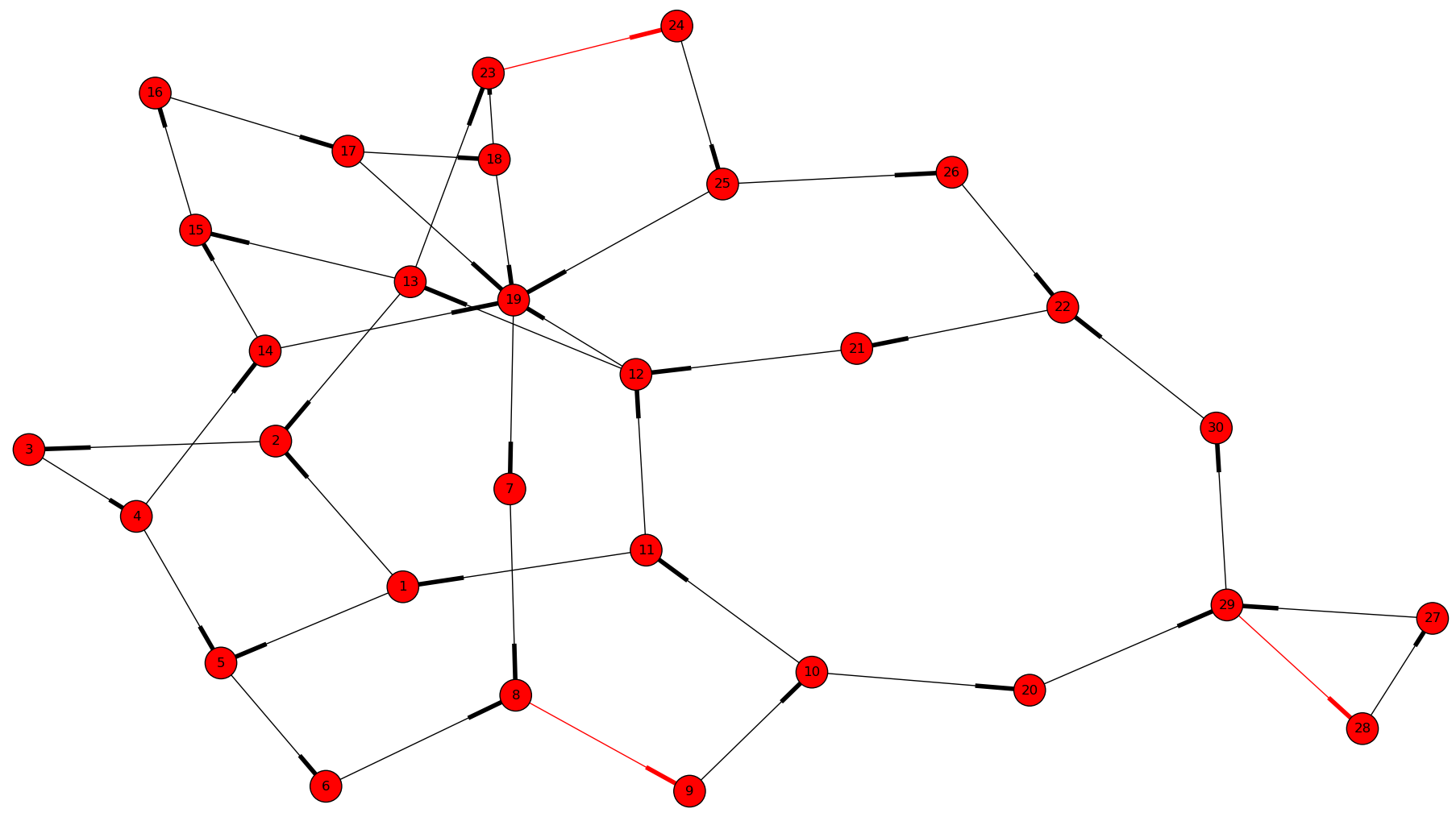
The 3 red edges form a minimum feedback arc set of the directed graph
Both a greedy heuristic and an exact algorithm has been implemented to solve the feedback arc set problem for weighted directed graphs.
Future work
Establishing a benchmark suite
Finding the optimal solution to tearing is NP-complete and approximation resistant. Therefore, a comprehensive benchmark suite has to be established, and then the various heuristics can be evaluated to see which one works well in practice. The COCONUT benchmark suite will be used for evaluating heuristics that do not require the natural block structure. I hope to receive help from the Modelica community to establish a test set where the natural block structure is available. Dr.-Ing. Michael Sielemann (Technical Director for Aeronautics and Space at Modelon Deutschland GmbH) has already offered his kind help.
Integration into Modelica tools
The implemented algorithms should be integrated into state-of-the-art Modelica tools. At the moment, a major obstacle is the inability to recover the process graph in the general case, as discussed above at the naming convention workaround.
Improving numerical stability
Tearing can yield small but very ill-conditioned systems; as a consequence, the final reduced systems can be notoriously difficult or even impossible to solve. Our recent publications [1] and [2] show how this well-known numerical issue of tearing can be resolved. The cost of the improved numerical stability is the significantly increased computation time.
Our pilot Java implementation has shown that it is crucial
- to design a convenient API for subproblem selection (roughly speaking: to be able to work with arbitrary number of diagonal blocks, ordered sequentially),
- to generate C++ source code for efficient evaluation of the subproblems (the residual and the Jacobian of the blocks),
- that the generated source code works with user-defined data types (and C++ templates do).
The next item on the agenda is to create a Python prototype implementation that meets all these requirements.
Source code generation for reverse mode automatic differentiation
The Jacobian is required when solving the subproblems with a solver like IPOPT. Generating C++ source code for evaluating the Jacobian of the subproblems is certainly not the main difficulty here: The primary challenge is to design an API that makes it easy to work with subproblems, and that makes the interfacing with various solvers only moderately painful.
I am not aware of any automatic differentiation package that would fulfill the requirements listed above, so I have set out to write my own. The diagonal blocks of the Jacobian will be obtained with reverse mode automatic differentiation. For example, for the expression
exp(3*x+2*y)+4*z
the following Python code is generated (hand-edited to improve readability)
# f = exp(3*x+2*y)+z
# Forward sweep
t1 = 3.0*x + 2.0*y
t2 = exp(t1)
f = 4.0*z + t2 - 1.0
# Backward sweep
u0 = 1.0
u1 = 4.0 * u0  # df/dz = 4
u2 = u0
u3 = t2 * u2
u4 = 3.0 * u3  # df/dx = 3*exp(3*x+2*y)
u5 = 2.0 * u3  # df/dy = 2*exp(3*x+2*y)
This code was automatically generated with the sibling package SDOPT.
The templated C++ version of this code will greatly benefit from code optimization performed by the C++ compiler, especially from constant folding and constant propagation. I expect the generated assembly code to be as good as hand-written.